|
Private |
E-textile Based Imaging Array: Phase Three
IntroductionThis web page describes the work done on the third phase of the project and the results obtained. We have implemented a new routing algorithm in view of the limitations of the flooding algorithm. We have also decided to use two separate routing algorithms for the two steps in the sensor array algorithm. The baseline model will also be modified such that only designated nodes will form the sensor image.
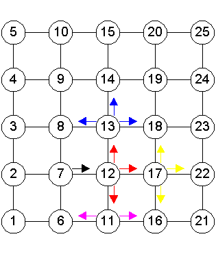
Routing AlgorithmsFlooding AlgorithmThe flooding algorithm was intended to be used for routing of the neighbor-ID data during Step 2, as well as sensor data during Step 3 of the sensor array algorithm, to pass data from each node to every other node. Each time a node receives a packet, it will retransmit to its other neighbors, except the one that it received the packet from. This is shown in Figure 1. Node 12 receives a packet from Node 7. Besides utilizing the information itself, it will retransmit the packet to Nodes 11, 13 and 17, which will then retransmit to their respective neighbors.
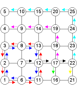
The “Ring” Algorithm Referring to Figure 2, suppose Node 17 wishes to send a packet
to every other node in the network. It will send the packet to Node
12. Upon receiving the packet from 17, Node 12 will retransmit the
packet through the ring formed by Nodes 13, 8, 3, 2, 1, 6, 11 and
12. The packet will be passed in both clockwise and counter clockwise
directions through the ring and back to Node 12 (blue arrows and
red arrows). Upon receipt of a packet in the ring, each node will
just pass it on in the same direction. When the same packet gets
back to Node 12, it will not retransmit again, since it is the originator
of the packet in the ring. Thus we see that Node 12 is both the
source and sink of the packet in the ring. Node 12 will also pass
the packet to Node 17 to form a second outer ring. Note that this
ring is, however, only a partial ring, terminating at Nodes 4 and
16. Thus in this case, 4 and 16 are the sinks. Node 17 will further
pass the packet to Node 22, to form a third level ring. Again this
is a partial ring, with Nodes 5 and 21 acting as the sinks.
Note in this case that Node 7 cannot just send the packet to Node 2, since it will not get propagate beyond the first level ring. Also, it is necessary send to both Nodes 12 and 8 in order to achieve redundancy in the outer rings. Advantages of “Ring” algorithm 2) Reduce traffic
Change to Baseline ModelThe ring algorithm has shown to have better performance than the flooding algorithm in the distribution of neighbor-ID information (Step 2 of sensor array algorithm), in terms of the time required for each node to form up the ID map. It also shows better performance in distribution of sensor information (Step 3 of sensor array algorithm). Although the image forming was still not complete, the nodes are able to form a larger image than when the flooding algorithm is used. However,
it is noticed that the images formed are “patchy” due
to large difference in delays. This means that information in the
nodes is not updated at the same rate, or at least a close enough
rate. Information for some node in the image may be very “old”
compared to other nodes. The Fixed Routing Algorithm
Current StatusThe ring algorithm has been implemented and tested.
Next PhaseThe next phase will be to implement the fixed routing algorithm and to start looking at the power issues.
ConclusionDue to the limitation of the existing routing flooding algorithm, a new Ring algorithm was conceived and implemented. The baseline model will be modified slightly such that only a designated node will form the sensor image. Also, two separate routing algorithms will be used for the two steps. The ring algorithm will be used for Step 2 for the passing of neighbor-ID data. A new fixed routing algorithm will be implemented for the routing of sensor information in Step 3.
References[1] “A Survey of Technologies for Smart Fabrics(Computational Textiles), DRAFT, Summer 2001”, Phillip Stanley-Marbell[2] “Project proposal, E-Textile-based Ultra-sound Imaging Array”, Seng Teck, Sing & Chee Wan, Teng [3] “Project Report Phase 1, E-Textile-based Ultra-sound Imaging Array”, Seng Teck, Sing & Chee Wan, Teng [4] “Project Report Phase 2, E-Textile-based Ultra-sound Imaging Array”, Seng Teck, Sing & Chee Wan, Teng [5] “Myrmigki Simulator Manual, Release 0.1.ece743”, Philip Stanley-Marbell. |
||||||||||||||||||||||||||||||||||||||||||||||||||||||||||||||||||||||||||||||||||||||||||
|
|||||||||||||||||||||||||||||||||||||||||||||||||||||||||||||||||||||||||||||||||||||||||||