E-textile Based Imaging Array: Phase Two

Introduction

This web page describes the work done on the second phase of the project and the results obtained. We have successfully resolved the problems we experienced in Phase 1. Using token-based network control, we were able to eliminate frame collisions. All the nodes in the array have been able to construct the ID map of the entire array. However, the sensor image has not been formed up in any of the nodes as each node was not able to propagate its data beyond its neighboring nodes, potentially due to link faults.

Work Done

Resolving Outstanding Issues from Phase 1

Frame collision
This happened when all the nodes attempt to transmit at the same time, which was highly likely given that they all run the same code. To solve this problem, we tried a random back-off algorithm to randomize the transmission so that frame collision is minimized. Unfortunately, we found that the random back-off strategy did not really help. While it did help to minimize the frame collision, the overall transmission time increased and it took a much longer time to complete the ID map construction. We then implemented a token-based method of network control. A token is passed between the two nodes. Only the node with the token can transmit and after it transmits, the token is passed to the other node. This approach proves to be a more efficient communication control, as frame collisions were virtually eliminated, since at any one time, only nodes having the token for a particular network segment could transmit.

Nodes “killed”
The reason was traced to the configuration file. All the boundary nodes were instantiated with some interfaces not attached to any network segments. Thus, when the nodes tried to transmit on these interfaces during a broadcast, the simulator would signal a fatal error and kill the node. Extra network segments were configured to fill this gap. After configuration file was fixed, the nodes were no longer “killed” by the simulator. The simulation continued to run and the nodes could complete the detection of their neighbors and other nodes in the map.

“Trying to draw water from empty well” syndrome
This was a message that was displayed repeatedly during the simulation. This seems to be related to the frame collision problem. The message no longer appears when the frame collision problem was resolved.

Unable to progress beyond “identify neighbors” stage
Some nodes were not able to complete the neighbors’ ID detection, while some began broadcasting their neighbors’ information. Due to the “killed” nodes and frame collision, the nodes were not able to construct the ID map and begin transmission of sensor data. With the frame collisions and “killed” nodes taken care of, all the nodes are able to reach the third stage, when they start transmitting their sensor data.

Other Problems Arising in Phase 2
During the simulation in Phase 2, we experienced loss of tokens/messages even when there is no collision. The current configuration simulates an “ideal” network i.e. all links are perfect. However, it seems that it is possible for messages and tokens to be lost. When this happen, the communication between two nodes stop because both are waiting for the token in order to transmit. The reason for the loss is not very clear, but it probably has to do with the changing of network interface during transmission or receipt of data.

In phase 2, all the nodes have started to transmit sensor data after they complete the ID map. However, it seems that the data of each node does not propagate beyond its neighboring nodes. We have managed overcome the problem of lost tokens by implementing a time-out for nodes waiting for the token. Thus a node will not wait infinitely for a token. However, it appears that the link failure rate is very high. Apparently, it seems like we already have a reliability problem.

Current Status

In phase 2, we managed to get the nodes to complete the construction of the ID map, which is a critical portion of the algorithm. However, the nodes were not able to receive the entire image.

On the simulation aspect, the configuration script for the imaging array setup is complete. Using the simulator’s “dumppwr” commands, we were able to show the power statistics of the individual nodes, although at this point of time, the power data is not too meaningful.

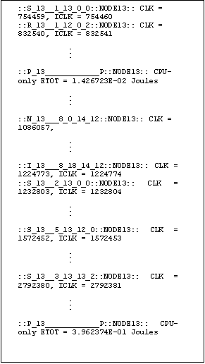
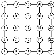
Log Files

During the simulation, every node outputs to an individual log file. Figure 1 shows a typical log file. The file specifically belongs to Node 13 (the complete log file for Node 13 can be found in the “Project Files” section). Figure 2 shows that distribution of the Node IDs. Note that although the IDs have been regularly distributed in this case, the algorithm does not assume that to be the case. Any distribution of IDs will work.

Figure 1
Typical log file of a node.
Note that although the IDs have been regularly distributed in this case, the algorithm does not assume that to be the case. Any distribution of IDs will work.

A typical line in the log file consists of three parts separated by “::”. The first part is output by our program to track the progress of the of the node
There are generally three types:

1) R_n__a_b_c_d: where
n : node number
a : message type
b : sending node number
c : origin node number
(0 for message type 1, 2, 4)
d : direction (0-3, see Figure 3)

R : Receive
S : Transmit
RS : Re-send

Purpose : to track the messages sent and received by the node
2) N_n__a_b_c_d: where
a, b, c, d : neighbor node ids
N : is for Neighbors not known
I : I is for Neighbors known or declared dead

Purpose : to signal the completion of the neighbor identification stage.
3) P_n____________P: where
n : node number

Purpose : To output the energy consumed by the node.

The second and third parts are generated by the simulator, denoting the node number and clock counts (for types 1 and 2) or energy consumed (for type 3).

Looking at Figure 1, we can see that Node 13 started off by broadcasting its own ID (sending a message Type 1). As it receives ID data from its neighbors, e.g. a Type 1 message from Node 12, it will update its own ID map. When it has collected information about all its four neighbors, it will indicate this by an 'I' printout with its neighbors’ IDs. Then, it will start to broadcast all its neighbors IDs (Type 2 message). If it receives a similar message (i.e. Type 2), it will reroute the message (send as a Type 5 message) and update its own ID map. When it completes building the ID map, it will start to send out its sensor data (Type 3 message).


Figure 2 Node IDs	Figure 3 Representation of channel directions

Next phase

The next phase will be a continuation of the current phase. We will continue to refine the algorithm and simulation such the all nodes would be able to build up the image array. A major consideration would be the reliability of the network links.

We shall also look at the power consumption of implemented architecture and explore different ways to reduce power consumption.

Conclusion

In conclusion, we have successfully resolved the problems we experienced in phase 1. The imaging array is able to construct the ID map of the entire array. Using token-based network control, we were able to eliminate frame collisions. However, the sensor image cannot be formed up yet, potentially due to link faults in the network.

References

[1] “A Survey of Technologies for Smart Fabrics(Computational Textiles), DRAFT, Summer 2001”, Phillip Stanley-Marbell

[2] “Project proposal, E-Textile-based Ultra-sound Imaging Array”, Seng Teck, Sing & Chee Wan, Teng

[3] “Project Report Phase 1, E-Textile-based Ultra-sound Imaging Array”, Seng Teck, Sing & Chee Wan, Teng

[4] “Myrmigki Simulator Manual, Release 0.1.ece743”, Philip Stanley-Marbell.